Scientific Programming with Python

Magnetic Spins

Magnets are atomic lattices with unpaired electrons, producing a spin magnetic moment at each position of the lattice:

↑ ↑ ↑ ↑ ↑ ↑ ↑ ↑ ↑ ↑          ↑ ↑ ↑ ↑ ↑ ↓ ↓ ↑ ↑ ↑          ↑ → ← ↑ ↑ ↓ ← ↑ → →

↑ ↑ ↑ ↑ ↑ ↑ ↓ ↑ ↑ ↑          ↑ ↑ ↑ ↑ ↑ ↓ ↓ ↓ ↑ ↑          ↓ ← ↑ ↓ ← → ↓ ← → ↑

↑ ↑ ↑ ↑ ↑ ↑ ↑ ↑ ↑ ↑          ↑ ↑ ← ← ↑ ↑ ↑ ↑ ↑ ↑          ← ↓ → ↓ ← ↑ ← ↑ ← ↓

↑ ↑ ↑ ← ↑ ↑ ↑ ↑ ↑ ↑          ↑ ← ← ← ↑ ↑ → → → →          ↓ ← → ← ↑ ← ↓ → ↓ →

↑ ↑ ↑ ↑ ↑ ↑ ↑ ↑ ↑ ↑          ↑ ↑ ↑ ↑ ↑ ↑ → → → ↑          ← ↑ ↓ ↓ → ↑ ← → ↑ ↓

  Low Temperature             Medium Temperature            High Temperature

These spins are tiny magnets and like to align with each other, and collectively can add up to a macroscopically measurable magnetization, such as in the bar magnet at the right:

The higher the temperature, however, the more the thermal energy randomizes the spins, and the uniform alignment is broken up by patches of spins in other directions called domains, as in the red and green regions in the micrograph at the left.

Above a critical temperature there is no longer a dominant magnetic direction, and the domain magnetizations cancel each other out.

At infinite temperature the spins are completely random in their orientation even over short distances.

We can describe the tendency of the spins to line up in terms of the (potential) energy of the spin interaction. Over the entire lattice of size N it is given by

E = – Σ_i≠j J_ij s_i·s_j

where J_ij is a positive coupling constant that incorporates the magnetic moment. Then,

• an alignment of the spins will produce a positive dot product and lower the energy, which is a more favorable state;
• an anti-alignment of the spins will produce a negative dot product and increase the energy, which is a less favorable state.

Complete spin alignment will have a large negative energy, while thermally randomized spins will have a higher energy near zero.

To simplify the model we can:

• establish a single z axis so that the spins in the vector dot product s_i·s_j can be replaced by their z-component s_i = ±1 ;
• limit the range of the interaction to only nearest-neighbor pairs, which can be written into the sum and allowJ to be a single value.

The energy thereby becomes

E = –J Σ_nn s_is_j

And we can represent the atomic lattice by an array of ±1 values:

  1 -1 -1  1  1 -1  1  1  1 -1
 -1 -1 -1  1 -1 -1 -1  1  1  1
  1 -1  1  1 -1  1  1 -1 -1  1
 -1 -1  1 -1  1  1 -1 -1  1  1
 -1 -1 -1  1 -1  1  1  1  1 -1
  1 -1 -1  1 -1  1  1  1  1  1
  1 -1 -1 -1  1 -1 -1 -1 -1 -1
 -1 -1  1 -1 -1 -1  1 -1 -1 -1
 -1 -1  1  1 -1 -1 -1 -1 -1  1
 -1 -1  1  1 -1 -1 -1  1 -1  1

This is known as the Ising Model of magnets, and as we will see it retains their basic characteristics.

When the spins substantially align, there will be a measureable magnetization:

M = (1/N)∣Σ s_i∣

• When T → 0, the spins completely align, and E → –2NJ and M → 1.
• When T → ∞, the spins will be randomly oriented, and E → 0 and M → 0.

The magnetization is an example of an order parameter, which we can use to monitor the system order.

Spyns

Not surprisingly, we can implement an Ising system and calculate its magnetization using Python.

We’ll use a two-dimensional lattice of size N = L × L:

L = 10
N = L**2

NumPy can define arrays with preset values in a number of ways. For example, to create a system at zero temperature, all spins aligned, we use:

import numpy as np
spins = np.ones((L,L), int)
print(spins)

⇒ 

[[1 1 1 1 1 1 1 1 1 1]
 [1 1 1 1 1 1 1 1 1 1]
 [1 1 1 1 1 1 1 1 1 1]
 [1 1 1 1 1 1 1 1 1 1]
 [1 1 1 1 1 1 1 1 1 1]
 [1 1 1 1 1 1 1 1 1 1]
 [1 1 1 1 1 1 1 1 1 1]
 [1 1 1 1 1 1 1 1 1 1]
 [1 1 1 1 1 1 1 1 1 1]
 [1 1 1 1 1 1 1 1 1 1]]

The first argument to ones() is the size of the lattice, as an n-tuple for an n-dimensional lattice.

The second argument sets the data type, in this case NumPy integers (otherwise it would produce a float).

The magnetization will tell us the degree of order in the model:

M = lambda : np.absolute(np.sum(spins))/N
print('M = ', M())

⇒ 1.0

Perfectly ordered, by design!

Warning: in Python 2.x, you’ll want to use float(N) in the above expression to avoid integer truncation.

The function np.sum() simply adds together all elements of the array it’s handed as an argument.

To create a system at infinite temperature, with a random distribution of values, we can use a subset of NumPy tools, numpy.random, that provides random number generators:

import numpy.random as npr
spins = npr.randint(0, 2, (L,L)) * 2 - 1
print(spins)

⇒
[[ 1  1  1  1  1 -1 -1 -1 -1  1]
 [ 1 -1  1  1 -1  1 -1 -1  1 -1]
 [ 1 -1 -1  1  1 -1  1  1  1  1]
 [-1  1  1  1  1  1 -1 -1 -1 -1]
 [-1 -1 -1  1 -1 -1 -1  1  1 -1]
 [-1  1  1 -1 -1 -1  1  1 -1  1]
 [ 1  1 -1 -1  1  1  1 -1  1  1]
 [-1  1  1 -1  1 -1  1  1 -1 -1]
 [ 1 -1  1  1 -1 -1  1 -1  1 -1]
 [-1 -1  1  1 -1  1 -1  1  1 -1]]

The first two arguments to randint() provide the range of integer values, minimum (inclusive) to maximum (exclusive), here producing values in the range (0, 1).

The third argument to randint() is the size of the lattice, again as an n-tuple for an n-dimensional lattice, here (L, L).

The result is a NumPy array of integers (0, 1), which allows broadcast calculations, here multiplication by 2 and then subtraction of 1 to produce the desired values of (–1, 1).

The magnetization is close to zero, as it should be for a completely disordered state:

print('M = ', M())

⇒ M = 0.06

It will never be precisely zero because it’s defined here, essentially, as the standard deviation of the average spin, but the larger the lattice we choose, the closer to zero it will be:

M = (1/N)∣Σ s_i∣~ (1/N)×N^1/2 ~ 1/N^1/2

So for N = 100, M ~ 0.1, as seen in the code snippet above.

Spyn Statistics

For a given temperature, how can we put this system in an equilibrium state so that we can calculate its order parameter? First we better define what we mean by “equilibrium”.

Statistical mechanics tells us that, for a system in equilibrium at a temperature T, representing a bath of thermal energy that randomizes the spins, the probability of a particular configuration of the spins is proportional to its Boltzmann factor:

P({s_i}) ∝ exp(–E/kT)

where the Boltzmann constant k “converts” temperature to a corresponding energy.

Clearly the lowest energy state will have the highest probability.

For the Ising Model:

P({s_i}) ∝ exp(–(–J Σ_nn s_is_j)/kT)
        = exp(β Σ_nn s_is_j )

where β = J/kT varies between ∞ and 0 as the temperature T varies between 0 and ∞.

In particular,

• When T → ∞ and β → 0, the exponential is equal to 1 for every pair of spins no matter what their orientation, meaning all states are equally likely, and there will be just as many “up” spins as “down” spins, on average.
• When T → 0 and β → ∞, the exponential is largest when the spins are all +1 or all –1, i.e. they all line up in one of those two directions.

Now consider an individual spin s_i and its neighbors s_inn; it has an energy relative to its neighbors of

E_i = –(J /2) s_i Σ_nns_inn

where the factor of 1/2 avoids double-counting the energy once we include the neighboring spins. It’s helpful to define a spin sum S_i as:

S_i = s_iΣ_nns_inn

E_i = –(J /2)S_i

The probability of a particular microstate s_i given neighbors s_inn is then:

P(s_i|s_inn) ∝ exp(–E_i/kT)
          = exp((β/2)S_i)

Distinct examples of the individual spin sum, energy, and probability are:

We can again see that:

• when the spins are less aligned, S_i < 0 and E_i > 0 and P(s_i|s_inn) < 1;
• when the spins are more aligned S_i > 0 and E_i < 0 and P(s_i|s_inn) > 1.

In addition, note that flipping the central spin will always invert the signs of S_i and E_i.

Now suppose we were to flip the central spin and this lowered the energy, e.g. we went from the second (blue) configuration in the table above to the last (pink) configuration. The spin sum is higher and the probability is also higher.

On the other hand, if flipping the central spin increased the energy, e.g. going from the last (pink) configuration to the second (blue) configuration, the spin sum will be lower and the probabilty will also be lower.

When in equilibrium the spins will flip back and forth over time, driven by the random energy of the temperature bath. However, on average, the system retains its state, in particular its degree of order. This means that the probability P of a microstate times the rate of transition W out of that microstate must be the same as the reverse process, i.e. over time the transition probabilities are equal:

P(s_i|s_inn)W(s_i → –s_i) = P(–s_i|s_inn)W(–s_i → s_i)

This condition is known as detailed balance, and is what we mean when we say a system is in equilibrium.

Detailed balance can also be used to drive a nonequilbrium system to equilibrium by flipping spins in a compatible manner, and this is the key to simulating such a system.

The ratio of the two transition rates is given by

W(–s_i → s_i)/ W(s_i → –s_i) = P(s_i|s_inn)/P(–s_i|s_inn)
                        = exp((β/2)S_i) / exp(–(β/2)S_i)
                        = exp(βS_i)

Suppose flipping the spin s_i → –s_i lowers the energy; again this means that initially E_i > 0 and S_i < 0. Because only the above ratio is important, we can choose this transition rate equal to 1, i.e. the spin will always flip:

W(E_high → E_low) = 1

Consequently, when flipping the spin s_i → –s_i increases the energy, initially E_i < 0 and S_i > 0, we must have

W(E_low → E_high) = exp(–βS_i) < 1

and the spin only has a fractional probability of flipping.

Increasing the energy is therefore less likely than decreasing it, and after repeated flipping attempts the lower energy state will become the most probable state, so that a nonequilbrium system must approach equilibrium over time.

Monte Carlo Simulations

Because of the randomizing effect of thermal energy and the probabilistic nature of the system energetics, we can use random numbers to equilibrate a system.

The Monte Carlo Procedure

Suppose we start with a system of spins at infinite temperature, which means they are randomly either ±1. We then instantaneously lower the temperature, a process known as quenching, and allow the system to equilibrate, or anneal.

Alternatively, for low temperatures, we can start with a system at zero temperature, with a uniform distribution of either +1 or –1, and then instantantaneously raise the temperature and allow it to equilibrate.

We can simulate such systems as follows:

1. Generate a lattice with the known initial configuration;
2. Randomly pick a spin;
3. Calculate its spin sum S_i = s_iΣ_nns_inn;
4. If S_i is less than or equal to zero, we flip it, since W(E_high → E_low) = 1;
5. Otherwise, calculate W(E_low → E_high) = exp(–βS_i);
1. Calculate a uniformly distributed random number 0 ≤ R < 1 and compare it to W;
2. If R < W, flip the spin (because a small transition rate W means a low probability of flipping);
6. Return to (2) and repeat until the system equilibrates.

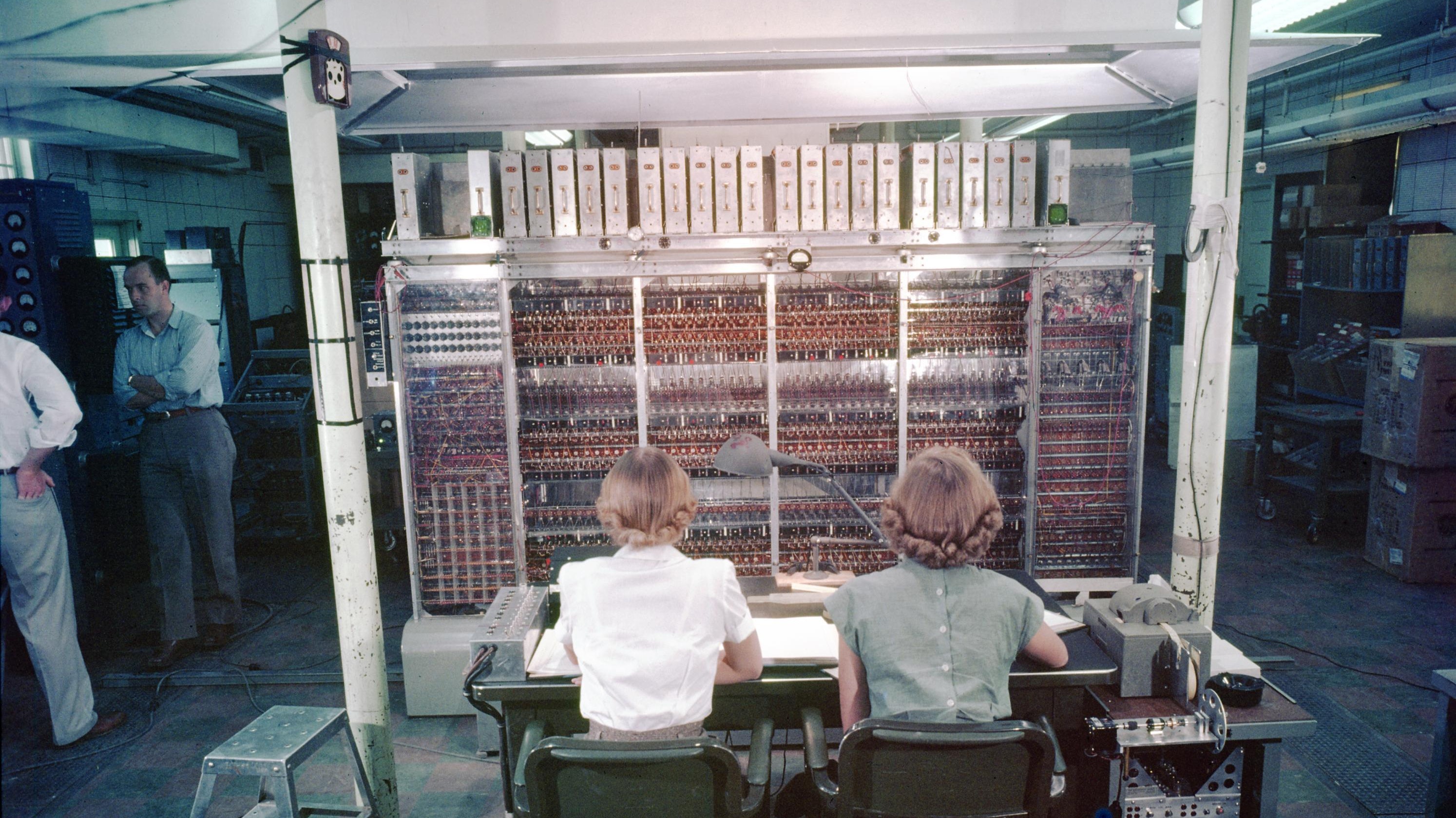
This Monte Carlo procedure is a standard practice in statistical science as a way to calculate the properties of complex systems. It is sometimes called Markov-Chain Monte Carlo (MCMC), since each state in the calculation depends only the immediately previous state.

It is also often referred to as the Metropolis Algorithm, after the first author of the 1953 paper Equation of State Calculations by Fast Computing Machines (who were listed in alphabetical order). However, the second author, computational physicist Arianna Rosenbluth, is credited with the actual implementation of the algorithm on one of the room-sized computers of the time, the MANIAC I at Los Alamos Scientific Laboratory in New Mexico:

The Monte Python Simulation

We’ll save the previous code in a file named ising.py!

import numpy as np
import numpy.random as npr
L = 10
N = L**2
M = lambda : np.absolute(np.sum(spins))/N
spins = npr.randint(0, 2, (L,L)) * 2 - 1
# More code here.
print(spins)
print('M = ', M())

We’ll also set a relatively large value of β that should produce some amount of ordering since it corresponds to a low temperature:

beta = 2

Now the next steps will take place in a loop after generating the spins, starting by randomly picking an initial spin, as sequential picking of spins would generate spatial correlations:

i = 0
while i < N :
    i += 1
    s = tuple(npr.randint(0, L, 2))

This last line returns two values in the range (0, L–1) as a NumPy array. It is converted to a tuple s=(sx, sy), indices into the array spins.

 1 -1 -1 sl  s sr  1 sb  1 -1
-1 -1 -1  1 sb -1 -1  1  1  1
 1 -1  1  1 -1  1  1 -1 -1  1
-1 -1  1 -1  1  1 -1 -1  1 st
sr -1 -1  1  1 st  1  1 sl  s
 1 -1 -1 -1 sl  s sr  1  1 sb
st -1 -1  1 -1 sb -1 -1 -1 -1
 s sr  1 -1 -1 -1  1 -1 -1 sl
sb -1  1  1 -1 -1 -1 st -1  1
-1 -1  1  1 st -1 sl  s sr  1

Now locate the indices of the adjacent spins, left, right, bottom, and top:

(sx, sy) = s
sl = (sx-1, sy)
sr = ((sx+1)%L, sy)
sb = (sx, sy-1)
st = (sx, (sy+1)%L)

When the spin s is at the left or bottom, one index is 0, and (0-1) ⇒ -1. But Python defines slices so that negative indices count backward from the largest value, i.e. the index -1 is equivalent to the index L-1, again wrapping around to the right or top edge.

On the other hand, when the spin s is on the right or top edge, one index is L-1, so that (L-1+1) ⇒ L, which Python treats as out-of-bounds. But we can use the modulus operator %, which provides the remainder when dividing two integers, to always produce a value within the range (0, L–1), specifically (L-1+1)%L ⇒ 0, wrapping around to the left edge or bottom edge.

These are known as circular boundary conditions and they help to reduce errors associated with finite lattice size.

Now calculate the spin sum S_i = s_iΣ_nns_inn:

    S = spins[s] * ( spins[sl] + spins[sr] + spins[sb] + spins[st] )

Finally test for the energy condition:

    if S <= 0 :
        spins[s] *= -1
    else:
        W = np.exp(-beta*S)
        R = npr.rand()
        if R < W : spins[s] *= -1

There is another random number generator here, rand(), which returns a floating point number between 0 (inclusive) and 1 (exclusive).

Once i reaches N, this loop terminates. We can calculate the matrix and magnetization at this time to see how they have changed, with the following statements that are not indented so they are only calculated once:

print(spins)
print('M = ', M())

Passing through the lattice once, on average, represents a single unit of time, since the entire lattice should have the chance to update once, no matter what its size. To run the loop for multiple units of time, define a number of time steps tmax and multiply it by the lattice size:

tmax = 100
i = 0
while i < tmax * N :
    i += 1
    s = tuple(npr.randint(0, L, 2))
    sl = (sx-1,sy)
    sr = ((sx+1)%L,sy)
    sb = (sx,sy-1)
    st = (sx,(sy+1)%L)
    S = spins[s] * ( spins[sl] + spins[sr] + spins[sb] + spins[st] )
    if S <= 0 :
        spins[s] *= -1
    else:
        W = np.exp(-beta*S)
        R = npr.rand()
        if R < W : spins[s] *= -1

Ensembles

The calculations above are for particular lattice sizes, and over particular periods of time. But they are also for particular configurations of spins, which have a probability

P({s_i}) ∝ Π_iexp(–E_i/kT) = exp(–Σ_iE_i/kT) = exp(–E/kT)

To calculate the order parameter M, we would use a weighted average over all configuration of the spins, known as an ensemble:

⟨M⟩ = Σ_i P_iM_i

Since a large lattice will have a huge number of configurations, 2^N, it’s impractical to calculate every one.

However, a random selection of spins such as above can be repeated multiple times, and that should sample the configuration space. Each of the selected configurations will occur with its own relative probabilty, and after Z samples the average result should provide a good approximation, known as the sample mean:

⟨M⟩ = (1/(Z−1))Σ_Z M

(The factor of Z–1 occurs due to a loss of one degree of freedom in a sample.) We can therefore add a loop to the above spin sample that repeats, for example, Z = 100 times, and accumulate each of the “measured” magnetizations to calculate this mean.

We can also calculate the sample mean of the magnetization squared:

⟨M²⟩ = (1/(Z−1))Σ_Z M²

which allows the calculation of the sample variance of M around the mean, given by:

s_M² = (1/(Z−1))Σ_Z(M − ⟨M⟩)²
   = (1/(Z−1))Σ_Z(M² − 2M ⟨M⟩ + ⟨M⟩²)
   = ⟨M²⟩ − 2⟨M⟩² + ⟨M⟩² Z/(Z−1)
   = ⟨M²⟩ − ⟨M⟩²(Z−2)/(Z−1)

and the sample standard deviation of M around the mean, given by:

s_M = sqrt(⟨M²⟩ – ⟨M⟩²(Z−2)/(Z−1))

The standard error of the mean of M then follows according to the Central Limit Theorem and is given by:

σ_M = s_M / sqrt(Z−1)

All together, the code adds an extra loop for Z, with initializations beforehand, accumulations after each step, and final calculations afterward:

Z = 100
tmax = 100
m = 0     # to accumulate the magnetization
m2 = 0    # to accumulate the magnetization squared
Ms = ()   # to hold the individual magnetizations to display a histogram
z = 0
while z < Z:
    z += 1
    i = 0; 
    while i < tmax * N:
        i += 1
        s = tuple(npr.randint(0, L, 2))
        (sx, sy) = s
        sl = (sx-1, sy)
        sr = ((sx+1)%L, sy)
        sb = (sx, sy-1)
        st = (sx, (sy+1)%L)
        S = spins[s] * ( spins[sl] + spins[sr] + spins[sb] + spins[st] )
        if S <= 0 :
            spins[s] *= -1
        else:
            W = np.exp(-beta*S)
            R = npr.rand()
            if R < W : spins[s] *= -1
    mi = M()
    Ms += (mi,)
    m += mi
    m2 += mi**2
Mavg = m / (Z-1)    # Average magnetization across the ensemble
M2avg = m2 / (Z-1)  # Average magnetization squared across the ensemble
sM = (M2avg - Mavg**2 * (Z-2)/(Z-1))**0.5  # Sample standard deviation of M around the mean
sigmaM = sM/(Z-1)**0.5  # Standard error of the mean of M

Accumulating the magnetizations in a tuple Ms also allows us to display a histogram of their distribution, to demonstrate its standard deviation:

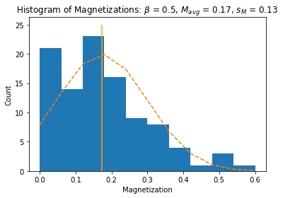
import matplotlib.pyplot as plt
figure, axes = plt.subplots()
n, bins, patches = axes.hist(Ms, 10)    # the histogram of the data in 10 bins
# add a 'normal' fit curve
y = ((1 / (np.sqrt(2 * np.pi) * sM)) *
     np.exp(-0.5 * (1 / sM * (bins-Mavg))**2))
y *= Z/np.sum(y)   # scale to match total
axes.plot(bins, y, '--', color='orange')
axes.vlines(Mavg, 0, 25, color='orange')
axes.set_xlabel('Magnetization')
axes.set_ylabel('Count')
axes.set_title(r'Histogram of Magnetizations: $\beta$ = ' + str(beta) + \
             ', $M_{avg}$ = ' + str(round(Mavg,2)) + ', $s_M$ = ' + str(round(sM,2)))
plt.show()
plt.close()

The standard deviation sM is visible here as the approximate width of the distribution to either side of the mean. The standard error of the mean σM is much smaller, by a factor of 1/√(Z–1), reflecting its relative stability due to the central limit theory.

The Amherst College High-Performance Computing System

Larger lattices can take a long time to process in the loop above, and they must then be averaged over a number of different configurations. While the script above should run well in Spyder, it will be very slow overall.

We can therefore turn to the Amherst College High-Performance Computing System, which provides a CPU cluster with 1024 CPU cores on 16 Unix computers, and has Python already installed.

On the CPU cluster we can run a number of calculations, or jobs, on these multiple cores and for longer periods of time.

Cluster jobs are prepared, tested, and submitted on an entry computer or login node, which you can access over the Internet from on-campus or while using a virtual private network (VPN) to appear to be on-campus. The HPC system’s login nodes are accessed via the domain name hpc.amherst.edu, or simply hpc.

General instructions for using the HPC system can be viewed in a web browser at https://hpc.amherst.edu/.

Python Scripts on the HPC System

Once you’ve mapped a network drive to your local computer as in Procedure 2, you can also use the Spyder IDE to read and write files on it.

When running your script on the HPC system, there are a few changes you’ll want to make so that it works more simply with Unix and the HPC system’s job management software.

One additional useful capability is to be able to hand your executable one or more arguments that could have different values for different jobs in the HPC system.

In Unix, such command-line arguments are typed following the initial command and separated by spaces, e.g.

./ising.py 1

where 1 might be a specific value of a variable such as beta.

If you import the “system” or sys module into your executable:

import sys

then you will have access to command-line arguments, passed to your executable as a list of strings:

sys.argv

⇒ ['./ising.py', '1']

beta = float(sys.argv[1])

⇒ 1.0

Note that item 0 in this list is set to the command you used to run the executable.

In general you will want to test to make sure that the expected number of arguments are provided, and either set a default value for missing arguments or exit the program with an error message (another function provided by the sys module):

if len(sys.argv) < 2 :
    sys.exit('Usage: ' + sys.argv[0] + ' beta')
else:
    beta = float(sys.argv[1])

Then when running the executable without arguments:

./ising.py

⇒ Usage: ./ising.py beta

If you need to engage in more complicated argument-list processing, especially if you want to include options like -t (e.g. to allow for keyword rather than positional arguments), take a look at the getopt module.

One other important change for your executable is to format its output to make it easier to analyze large quantities of data; most simply, you can write comma-separated values so that the results of different jobs can all be concatenated together into a table:

print('L,Z,beta,Mavg,sM,sigmaM')
print('%d,%d,%0.2f,%0.3f,%0.3f,%0.3f' % (L,Z,beta,Mavg,sM,sigmaM))

⇒
L,Z,beta,Mavg,sM,sigmaM
10,100,10.00,0.77,0.37,0.038

The Slurm Job-Management System

The Slurm job-management software provides an efficient means to control a project running on a large number of computers.

A set of related jobs are submitted as a cluster of jobs that are automatically distributed over any available computer cores.

By design CPU time is shared with other researchers; the general behavior is that newer clusters are given priority, and the longer they run the lower their priority becomes.

Along with your executable program, Slurm will need a batch file for each job cluster, which provides details on how to run each job, including any command-line arguments that might vary from job to job.

The basic structure of a batch file is a series of commands, one per line, usually key=value pairs that describe either global job properties or individual job properties, for example:

## Global job properties
universe     = vanilla
notification = error
notify_user  = username@amherst.edu
executable   = /mnt/scratch/username/ising/ising.py
requirements = (((Arch=="INTEL") || (Arch=="x86_64")) && (OpSys=="LINUX"))
priority     = 5

## Job properties
arguments = 0.1
initialdir = /mnt/scratch/username/ising/results/0
output = /mnt/scratch/username/ising/results/0/out
error  = /mnt/scratch/username/ising/results/0/err
log    = /mnt/scratch/username/ising/results/0/log
queue

## Job properties
arguments = 0.2
initialdir = /mnt/scratch/username/ising/results/1
output = /mnt/scratch/username/ising/results/1/out
error  = /mnt/scratch/username/ising/results/1/err
log    = /mnt/scratch/username/ising/results/1/log
queue
...

As with Python, a # introduces a comment.

The keyword universe describes possible modes of running your executable; when the jobs are independent of each other (don’t need to pass information amongst themselves), the proper value is vanilla. There are other possiblities for more specialized applications, e.g. for code compiled with parallel-processing libraries.

The keyword notification determines whether an e-mail will be sent for certain situations:

• complete (the default): upon job completion, whether properly or due to errors
• error: only when job errors occur
• never

The complete option is not generally recommended, because it can generate hundreds of e-mails, one for each job, which look like:

This is an automated email from the Slurm system
on machine "csc2-node01.amherst.edu". Do not reply.

Slurm job 150601.0
/mnt/scratch/username/ising/ising.py 0.1
has exited normally with status 0
....

If you set notification to something other than never, you should include your e-mail address using the notify_user keyword.

The keyword executable is the location of the application that Slurm is going to run.

The keyword requirements describes various node characteristics necessary for your application, in particular the hardware architecture (Arch) and operating system (OpSys), together known as the node platform. Since Slurm runs on heterogeneous equipment, but many applications cannot, this keyword is important to set properly, especially since the default platform characteristics are the same as the login node. The requirements can both be limited with an AND statement (&&) or expanded with an OR statement (||). For the Amherst College HPC system the value combination above describes all of its platforms, which all run the Linux operating system, but which are either AMD or Intel CPUs — and therefore run the same compiled binary code.

The keyword priority is any integer and is a relative priority for your own jobs — a lower priority, such as 0 (the default), will be run only after your other jobs with higher priority have run. This doesn’t effect job priority relative to other users, which is set by Slurm using its own algorithm.

The keyword arguments is a list of text values that will be handed to your application, e.g. ising.py 0.1.

The keyword initialdir is the working directory where each instance of the application will run and where its varying input and output files are or will be located. Keeping them in the same directory allows the app to read and write with local references no matter which instance it is. Common input files can be referenced either with full paths or with relative references, e.g. ../.. to refer to the base directory.

The keywords output, error, and log describe files to store, respectively, standard output from your application (what would appear as output if you ran it directly), any error messages that occur, and Slurm’s log of running the job providing information similar to the e-mail above.

The keyword queue tells Slurm to submit one job with the previous set of characteristics. You can then change a few of them for the next job, and queue that. The variant queue n submits n jobs all with the same characteristics, useful when other parameters are created randomly by the program.

There are many more commands that might occasionally be useful and that are described in the Slurm documentation.

Once you’ve created your batch file, use Slurm_submit to send your project to the Slurm job queue.

import os, math

# Create file references for this project:
projectName = 'ising'
baseDirectory = os.getcwd()
executable = baseDirectory + '/' + projectName + '.py'
commandFile = baseDirectory + '/' + projectName + '.sb'

# Write the global parameters needed for all jobs into the batch file: 
commands = open(commandFile, 'w')
commands.writelines(['## Global job properties\n',
	'universe =     vanilla\n',
	'notification = error\n',
	'notify_user  = username@amherst.edu\n',
	'getenv =       true\n',
	'executable =   ' + executable + '\n',
	'requirements = (((Arch=="INTEL") || (Arch=="x86_64")) && (OpSys=="LINUX"))\n',
	'priority =     5\n'])

# Create the results directory and limit accessibility to yourself with
# the permission rwx --- --- (0o700):
baseResultsDirectory = baseDirectory + '/results'
if not os.path.exists(baseResultsDirectory) : 
    os.mkdir(baseResultsDirectory, 0o700)

# Job arguments, here [0.1, 0.2, 0.3, …, 1.3, 1.4, 1.5]:
betaValues = [(x+1)/10 for x in range(15)] 
jobsCount = len(betaValues)

# Create a format string that will produce results directory names that 
# have a standard length for sorting purposes, e.g. 'results/%02d'
#  => 'results/00', ..., 'results/09', 'results/10', ..., 'results/99'
resultsDirectoryFormat = baseResultsDirectory + '/%0' + \
                         str(math.floor(math.log10(jobsCount - 1)) - 1) + 'd'

# Loop through the parameters to be passed for each job:
for job in range(jobsCount) :

    # Create the results directory for this specific job.
    resultsDirectory = resultsDirectoryFormat % job
    if not os.path.exists(resultsDirectory) : 
        os.mkdir(resultsDirectory, 0o700)

    # Write the arguments for this job.
    commands.writelines(['\n## Job properties\n',
    	'arguments = ' + str(betaValues[job]) + '\n',
    	'initialdir =   ' + resultsDirectory + '\n',
    	'output = ' + resultsDirectory + '/out\n',
    	'error = ' + resultsDirectory + '/err\n',
    	'log = ' + resultsDirectory + '/log\n',
    	'queue\n'])

commands.close()

chmod +x ising.sb

./ising.sb

ls results
⇒
00  01  02  03  04  05  06  07  08  09  10  11  12  13  14  15

#! /bin/sh
#SBATCH --ntasks=50
#SBATCH --output=ising-%j.out
#SBATCH --error=ising-%j.err

# Check for the results directory, and if it isn't present, create it:
if [[ ! -d 'results' ]]; then mkdir 'results'; fi

# Hand the python script to Slurm to run, each task on its own cpu, and wait for them to complete:
srun --overlap -o results/ising-%j-%2t.out -e results/ising-%j-%2t.err ./ising.py
wait